Contravariance and Covariance - Part 1
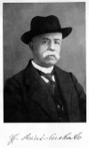
| Founders of Tensor Analysis | ||
|---|---|---|
 |
 |
|
| Gregorio Ricci Curbastro | Tullio Levi-Civita | |
In the design of computer languages, the notion of contravariance and covariance
have been borrowed from category theory to facilitate the discussion of type
coercion and signature. Category theory, on the other hand, borrowed and abstracted
the notion of contravariance and covariance from classical tensor analysis which
in turn had its origins in physics.
Unfortunately, the people who tend to be familiar with category
theory, and indeed tensor analysis, and the ideas of contravariance and covariance,
are more often mathematicians, and not usually computer scientists.
I therefore hope to give a gentle introduction to some of these ideas.
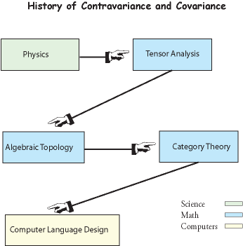 |
| Figure 1 The flow of ideas leading to the development and use of category theory in computer science. |
We begin with physics because the idea of contravariance and covariance
has its origins in the study of vectors. The concept of a vector has undergone a
great amount of refinement and generalization in its history. Depending on the mathematical
spaces one is considering, such generalization is necessary. But additionally, it
is also useful to have a variety of ways of thinking about the vector concept. To
quote Feynman:
"Theories of the known, which are described by different physical ideas, may be equivalent in all their predictions and hence scientifically indistinguishable. However, they are not psychologically identical when trying to move from that base into the unknown. For different views suggest different kinds of modifications which might be made and hence are not equivalent in the hypotheses one generates from them in one's attempt to understand what is not yet understood." -- Feynman [1]
"Theories of the known, which are described by different physical ideas, may be equivalent in all their predictions and hence scientifically indistinguishable. However, they are not psychologically identical when trying to move from that base into the unknown. For different views suggest different kinds of modifications which might be made and hence are not equivalent in the hypotheses one generates from them in one's attempt to understand what is not yet understood." -- Feynman [1]
(That is also a good quote to keep in the back of one's mind when we come to category theory.) Therefore, we will enumerate some of the common
vector definitions. However, no matter how much the concept is generalized, in engineering
and physics, the geometric notion of an arrow that obeys a superposition principle
is fundamental. And in mathematics, the algebraic notion contained in a linear vector
space, is fundamental. In both the arrow and vector space notions, there is a natural
idea of contravariance and covariance. In computer science, the concept of a vector
(i.e., an ADT) refers to a completely unrelated idea and in no way should be confused
with the concepts of vector we are considering here.
Vector Concept 1 - Directed Line Segment: The vector concept one first studies in school is usually that of an arrow,
or a directed line segment. Forces and displacements are examples of quantities that can be
modeled by directed line segments. Experimentally,
it is found that both forces and displacements can be combined graphically by the
parallelogram method of addition. The discovery of this method seems to have been
first made by the Dutch mathematician Simon Stevinus (1548-1620).
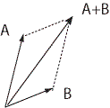
|
| Figure 2 Addition of vectors by the parallelogram method |
Abstracting, an elementary definition of a vector is that a vector
is an object that can be represented
by a directed line segment and that combines with other vectors via the parallelogram
method of addition. The magnitude of the vector is
given by the length of the arrow.
This definition is of great utility in physics and engineering,
but it is not capable of being used in more abstact spaces than Rn without
modification. However, those abstract spaces are typically manifolds, and
a manifold "locally looks like" Rn (where n is the dimension of
the manifold) So, even if we want to jump ahead to a more advanced definition, it
is quite useful to understand how vectors are defined in Rn.
Rectangular and Oblique Coordinates Systems in R2
Without loss of generality, we restrict our discussion now to mostly R2. Extending to Rn is not difficult, but complicates the example. Shown below is a rectangular coordinate system and the resolution of a vector A into its rectangular coordinates.
Without loss of generality, we restrict our discussion now to mostly R2. Extending to Rn is not difficult, but complicates the example. Shown below is a rectangular coordinate system and the resolution of a vector A into its rectangular coordinates.
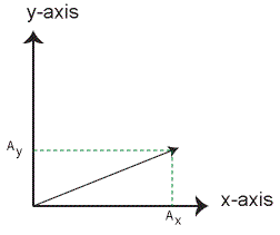 |
| Figure 3 Rectangular Components of Vector A |
In rectangular coordinates, the contravariant and covariant
components of a vector are usually the same, as will become clear later.
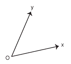
We now extend the class of coordinate systems to consider those systems whose axes are not perpendicular, or in other words, oblique coordinates. Let OX be a line through the points O and X, and OY be a line through the points O and Y, chosen so that the lines are not colinear and they meet at an oblique angle. Then, with O chosen as the origin, this constitutes an oblique coordinate system for R2.(Figure 4)
We now extend the class of coordinate systems to consider those systems whose axes are not perpendicular, or in other words, oblique coordinates. Let OX be a line through the points O and X, and OY be a line through the points O and Y, chosen so that the lines are not colinear and they meet at an oblique angle. Then, with O chosen as the origin, this constitutes an oblique coordinate system for R2.(Figure 4)
|
| Figure 4 An Oblique Coordinate System |
The parallel projection onto the OX axis gives the x coordinate, or abscissa, Ax,
of the vector A. The parallel projection onto OY gives the y coordinate, or ordinate,
Ay, of the vector A.(Figure 5)
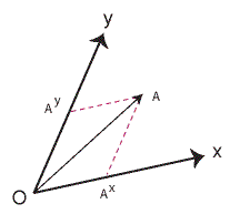 |
| Figure 5 Oblique Coordinates of Vector A |
The components Ax and Ay are called the
contravariant components of A. It is important to note
that x and y are not exponents, but their raised position relative to A is the standard
notation for contravariant components that is used to distinguish them from the
covariant components, which we will now introduce.
Reciprocal Lattice
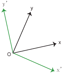
To define the covariant components of A, we have to introduce the concept of the reciprocal lattice. Rotating the x axis by 90 degrees counter clockwise gives the y'-axis of the reciprocal lattice, and rotating the y axis by clockwise by 90 degrees gives the x'-axis of the reciprocal lattice. The original coordinate system is called the direct coordinate system, or direct lattice. The reciprocal lattice is shown, in green, in figure 6.
|
| Figure 6 The Reciprocal Lattice in R2 |
To define the covariant components of A, we have to introduce the concept of the reciprocal lattice. Rotating the x axis by 90 degrees counter clockwise gives the y'-axis of the reciprocal lattice, and rotating the y axis by clockwise by 90 degrees gives the x'-axis of the reciprocal lattice. The original coordinate system is called the direct coordinate system, or direct lattice. The reciprocal lattice is shown, in green, in figure 6.
This
procedure works in R2only.
Generally in Rn, the reciprocal lattice is defined by introducing non-zero
"basis"
vectors, not necessarily of unit length, along each axis x1,...,xn.
(Because the number of axes can in general exceed the number of distinct letters
in the alphabet, we now switch to labeling the axis not as x,y,z but as x1,...,xn)
Let
e1 be a non-zero vector along the x1 axis, e2 a non-zero vector along x
2
axis,..., and en be a non-zero vector along xn
, then this set of vectors set {e1,...,en}
is a "basis" for the direct coordinate system. If we are given the basis, we can
form the coordinate axes, and vice-versa. The reciprocal lattice "basis" , {e1,...,en} then
is defined by the requirement
eiek cos[angle(i,k)] =1 if i=k, and 0 otherwise, where angle(i,k) is the angle between e i and ek.
eiek cos[angle(i,k)] =1 if i=k, and 0 otherwise, where angle(i,k) is the angle between e i and ek.
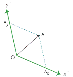 |
| Figure 7 Covariant Components of Vector A |
Having constructed the reciprocal lattice, the parallel projections of A onto the x'-axis and the y'-axis give the covariant components of A, as shown in Figure 7.
For completeness, it should be noted it is also possible to give an
interpretation of the covariant components as orthogonal projections on the direct
coordinate sytem, rather than parallel projections on the reciprocal lattice. In
fact, this interpretation was given by the founders Ricci and Lev-Civita. However,
this interpretation requires multiplication of the components by a factor,
which destroys the symmetry of the formulation.
The reciprocal lattice seems to have its origins in crystallography,
but it also has great application in solid state
physics.
Next Week -- Part 2 -- Contravariance and covariance in abstract vector spaces.
Vectors as elements of vector spaces, change of basis, multilinear algebra
References:
[1] Richard Feynman, The Development of the Space-Time View of Quantum Field Theory. Nobel Lecture, 1966.