Contravariance and Covariance - Part 3
Albert Einstein
Tensor Calculus
Vector Concept 3 -- Classical Tensor Analysis in Rn
Our transformations of coordinates have hitherto mostly involved constants
in the change of coordinates transformation matrix. We now extend the allowed transformations to include more
general functions, from which we
get yet another definition of a vector.
It will turn out, for general
non-cartesian coordinates, there are two possible transformation laws. One law describes
contravariant vectors, and the other covariant vectors.
While part 2 required some knowledge of algebra, this part will require some knowledge of
multi-variable calculus. For brevity, I give only the essential concepts. As a minimum,
some knowledge of the chain rule would be needed to follow along.
Curvilinear Coordinates
Let x1,...,xn be a rectangular coordinate system in Rn. (It should perhaps be remarked that it in general mathematical spaces, it is not always possible to find such a coordinate sytem. The existence of a global rectangular coordinate system is equivalent to assuming the space is Euclidean.) Consider the general transformation of coordinates to a new, not necessarily rectangular, coordinate system y1,...,yn:
Let x1,...,xn be a rectangular coordinate system in Rn. (It should perhaps be remarked that it in general mathematical spaces, it is not always possible to find such a coordinate sytem. The existence of a global rectangular coordinate system is equivalent to assuming the space is Euclidean.) Consider the general transformation of coordinates to a new, not necessarily rectangular, coordinate system y1,...,yn:
|
y1 = y1(x1,...,xn) ... ............... ... ............... ... ............... yn = yn(x1,...,xn) |
(Eq. 1) |
We require certain technical conditions in order that our new coordinate system be
well defined. In
particular, the transformation should be differentiable
and have a differentiable inverse. Sufficient conditions for this are
given by the implicit function theorem -- the Jacobian of the transformation
should be non-zero. The y-coordinate
system so defined
constitutes a curvilinear coordinate system.
Now that curvilinear coordinates have been introduced, we can consider transformations from one curvilinear coordinate system to a different
curvilinear coordinate system...
which brings us to the classical idea of a tensor and the corresponding definitions:
Scalar
A function f(x1,...,xn) is a scalar if under a change of coordinates (1), it does not change value.
In other words, if f′, or f prime, is the value in the new y-coordinate system (f prime is not the derivative!),
f′(y1,...,yn) =
f(x1,...,xn)
Typical examples of scalars are mass and temperature, which are independent of choice
of coordinates. A scalar is also called a tensor of rank 0
. Vectors, which we now define, are tensors of rank 1.
Contravariant Vector
A contravariant vector is a set of functions vk that, under a change of coordinates, transform as
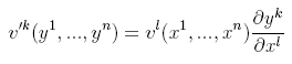
|
(Eq. 2) |
Covariant Vector
A covariant vector is a set of functions vk that, under a change of coordinates, transform as
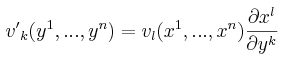
|
(Eq. 3) |
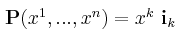
The origin of the above definitions may not at first be obvious. However, if we
expand the standard position "vector" P(x1,...xn) in the standard
rectangular coordinate basis {i1,...,in} ,the relation to our previous definitions becomes more apparent.
we see the rectangular basis "vectors", {i1,...,in},
are given by
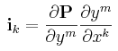
Now, changing coordinates to y-coordinate system, we find
Examining this equation for ik, we recognize
as the tangent vector to the ym coordinate curve. The set of vectors
gm are known as the curvilinear basis vectors for the y-coordinate
system, and form a basis for Rn (That they form a basis
is gauranteed by virtue of the fact that the Jacobian of the transformation is non-zero). Therefore, any vector v in Rn can be expanded as
The vk are the covariant components of v.
 |
(Eq. 4) |
 |
(Eq. 5) |
 |
(Eq. 6) |
 |
(Eq. 7) |
 |
(Eq. 8) |
The vk are the contravariant components of v.
Denoting the dual basis to the {gm} by {gm},
we can expand v in the dual basis as
 |
(Eq. 9) |
The vk are the covariant components of v.
It might come as a surprise that in the most general case in this definition, when
non-orthognal transformations are allowed, a finite directed line segment will not
in general obey the transformation laws (2) or (3) and so is NOT a vector.
However, infinitesimal directed line segments
are vectors.
This whole analysis has assumed the existence of a global rectangular coordinate system, or in other words, that the space we are considering is Euclidean. Easing this restriction, and considering non-Euclidean spaces, leads us to the study of vectors defined on more general spaces called manifolds.
Next week -- Vectors on Manifolds.